해당 내용은 coursera Andrew Ng교수의 Machine Learning강의 노트 정리
Trouble shooting
Hypothesis에 새로운 데이터를 적용했을 때 시도할 수 있는 방법들
- training example을 늘린다.
- feature갯수를 줄이거나 늘린다.
- polynomial feture를 사용한다. [주택가격예측 예에서]
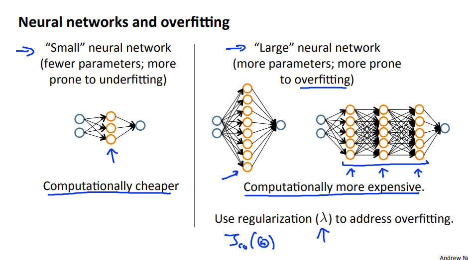
- $\lambda$를 줄이거나 증가시킨다.[정규화]
→ 진단을 통해 어떻게 성능 향상을 할 것인지 insight를 얻고 개선하는 것이 효율적
Evaluating Hypothesis
Data를 Training set과 Test set으로 나눈다.
Linear regression
- training data로부터 training error를 최소화하는 parameter$\theta$를 학습.
- test set으로 error를 계산.
$$ J_{test}(\theta)= \frac {1}{2m_{test}} \sum_{i=1}^{m_{test}}(h_{\theta}(x_{test}^{(i)})-y^{(i)})^2 $$
Logistic regression
- training data로부터 parameter$\theta$를 학습
- test set으로 error를 계산
$$ J_{test}(\theta)= -\frac{1}{m_{test}} \sum_{i=1}^{m_{test}}y_{test}^{(i)}logh_{\theta}(x_{test}^{(i)})+(1-y_{test}^{(i)})logh_{\theta}(x_{test}^{(i)}) $$
- classification error계산 [잘못분류된 것 =1, 잘 분류된것 =0]
$$ err(h_\Theta(x),y) = \begin {matrix} 1 &{if } \ h_\Theta(x) \geq 0.5\ and\ y = 0\ or\ h_\Theta(x) < 0.5\ and\ y = 1\newline 0 & otherwise \end {matrix}\\Test Error=\frac {1}{m_{test}}∑_{i=1}^{m_{test}}err(h_Θ(x_{test}^{(i)}), y_{test}^{(i)}) $$

서로 다른 모델을 평가하고 어떤 것이 Hypothesis에 적합한 것인지 선택하기 위해서 test data를 통해 선택하는 것보다 validation set을 통해 선택하고 test set을 통해 새로운 데이터의 error를 평가해야한다. 왜냐하면 test set을 통해 model을 택하였기 때문에 generalization error의 optimistic estimate가 되기 때문이다.

Train/ validation/ Test error
$$ J_{train}(\theta)= \frac{1}{2m_{train}} \sum_{i=1}^{m_{train}}(h_{\theta}(x_{train}^{(i)})-y^{(i)})^2\\ J_{cv}(\theta)= \frac {1}{2m_{cv}} \sum_{i=1}^{m_{cv}}(h_{\theta}(x_{cv}^{(i)})-y^{(i)})^2\\J_{test}(\theta)= \frac {1}{2m_{test}} \sum_{i=1}^{m_{test}}(h_{\theta}(x_{test}^{(i)})-y^{(i)})^2 $$
Training set을 통해 parameter를 학습하고 validation set을 통해 model을 선택한 후 test set으로 generalization error를 계산한다.
Bias VS Variance
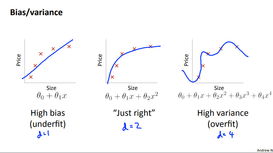

High bias[underfitting] : $J_{train}(\theta)$와 $J_{cv}(\theta)$ 모두 높다. $J_{CV}(Θ)≈J_{train}(Θ).$
High variance[overfitting: $J_{train}(\theta)$는 낮지만 $J_{cv}(\theta)$는 $J_{train}(\theta)$에 비해 훨씬 크다
Regularization


- Create a list of lambda [ ex, $\lambda ∈ \{0,0.01,0.02,0.04,0.08,0.16,0.32,0.64,1.28,2.56,5.12, 10.24\}$]
- Create a set of models with different degrees or any other variants
- Iterate through the $\lambda$s and for each $\lambda$ go through all the models to learn some $\theta$
- Compute the cross validation error using the learned $\theta$ (computed with $\lambda$) on the $J_{cv}(\theta)$ without regularization or $\lambda =0$
- Select the best combo that produces the lowest error on the cross validation
- Using the best combo $\theta$ and $\lambda$, apply on $J_{cv}(\theta)$ to see if it has a good generalization of the problem
Learning Curves

2차 함수를 hypothesis function으로 하는 예에서 만일 매우 적은 수의 데이터 (예: 1, 2 또는 3개 )에 대해 알고리즘을 훈련하면 항상 정확하게 해당 포인트에 닿는 2차 곡선을 찾을 수 있기 때문에 오류가 0개가 되기 쉽다. 그러나 훈련 세트가 커질수록 2차 함수에 대한 오차는 증가하다가 특정 m 또는 세트 크기 이후에 고정된다.

High bias : training error와 validation error 모두 크며 validation error 값이 더 이상 줄지 않는 pleatue 한 구간에 빠르게 도달하게 된다. ⇒ 더 많은 training data는 도움이 되지 않는다.
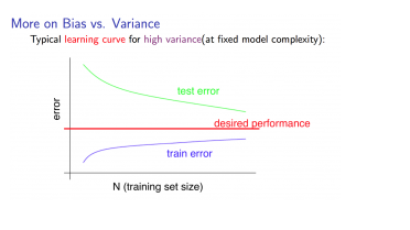
High variance: : training error와 validation error 간의 차이가 크며 데이터를 늘리는 것이 도움이 될 수도 있다.
What to next
- Getting more training examples: Fixes high variance
- Trying smaller sets of features: Fixes high variance
- Adding features: Fixes high bias
- Adding polynomial features: Fixes high bias
- Decreasing λ: Fixes high bias
- Increasing λ: Fixes high variance.
모형 복잡성 효과:
하위 다항식[낮은 모형 복잡성]: high bias and low variance, 모형의 적합도가 일정하지 않음
고차 다항식[높은 모델 복잡성]: training data 매우 잘 적합시키고 테스트 데이터를 매우 fit 하지 못하며 training data에 대해 low bias and high variance.
Refrenece
Machine learning , Coursera, Andrew Ng