해당 내용은 coursera Andrew Ng교수의 Machine Learning강의노트
Gradient Descent
cost function인 $J(\theta_0, \theta_1)$을 최소화 하기 위한 hypothesis function의 최적 파라미터값을 찾기 위해 gradient descent를 하게 된다.
$$ min_{\theta_0,\theta_1} J(\theta_0, \theta_1) $$
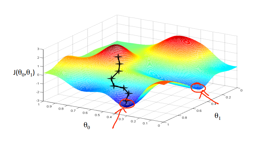
일반적으로 비용함수는 하나의 global minimun만 갖는 것이 아니라 여러 개의 local minimum을 가진다. 초기값이 어디인가에 따라서 local minimun으로 수렴하게 되거나 global minimum에 도달할 수 있기 때문에 초깃값의 설정이 중요하다.

Gradient descent algorithm
$$ \theta_j := \theta_j - \alpha \frac{\partial}{\partial \theta_j} J(\theta_0, \theta_1) $$
→ $\theta_0$과 $\theta_1$을 동시에 update 해야 한다.
correct update : simultaneous update
$$ temp0 := \theta_0 := \theta_0 - \alpha \frac{\partial}{\partial \theta_0} J(\theta_0, \theta_1) \\temp1 := \theta_1 := \theta_1 - \alpha \frac {\partial}{\partial \theta_1} J(\theta_0, \theta_1) \\ \theta_0 := temp0 \\ \theta_1 := temp1 $$
Incorrect :
$$ temp0 := \theta_0 := \theta_0 - \alpha \frac{\partial}{\partial \theta_0} J(\theta_0, \theta_1) \\\theta_0 := temp0 \\temp1 := \theta_1 := \theta_1 - \alpha \frac {\partial}{\partial \theta_1} J(\theta_0, \theta_1) \\ \\ \theta_1 := temp1 $$
Gradient descent - Intuition
$$ \theta_j := \theta_j - \alpha \frac{\partial}{\partial \theta_j} J(\theta_0, \theta_1) $$
$\alpha$: learning rate
$\frac{\partial}{\partial \theta_j} J(\theta_0, \theta_1)$: 편미분
파라미터 $\theta_1$에 대해서 cost function을 아래의 그래프 같이 나타낼 수 있다고 할 때,

편미분의 값이 양수이면 $\theta_1$의 값이 작아지도록 update가 되고 편미분의 값이 음수이면 $\theta_1$의 값이 커지게 된다.
learning rate의 값은 step size(보폭)으로 생각할 수 있다. 보폭이 작으면 gradient descent값이 작게 되고 minimum에 천천히 수렴하게 된다. 그러나 learning rate $\alpha$가 크면 minimunm에 수렴하지 못하고 오히려 발산하게 될 수도 있다.

learning rate $\alpha$의 값이 고정된 상수더라도 gradient descent는 local minimum값에 수렴할 수가 있는데 이것은 $\theta_1$이 update 되면서 편미분 값이 줄어들게 되고 자동적으로 gradient descent 값도 줄어들게 되어 학습을 진행하면서 learning rate을 줄여주지 않아도 된다.

local minimum에서의 편미분의 값도 0이 되기 때문에 현재 $\theta_1$이 local minimum에 있다면 $\theta_1$의 값은 더 이상 update 되지 않게 된다.
Gradient Descent for Linear Regression
Linear Regression
$$ h_{\theta}(x) = \theta_0 + \theta_1x \\ J(\theta_0,\theta_1) =\frac {1}{2m} \sum_{i=1}^{m}(h_{\theta}(x^{(i)}-y^{(i)})^2 \\ $$
$\frac {\partial}{\partial \theta_j} J(\theta_0, \theta_1) = \frac{\partial}{\partial \theta_j} \frac{1}{2m}\sum_{i=1}^{m}(h_{\theta}(x^{(i)}-y^{(i)})^2 \\=\frac{\partial}{\partial \theta_j} \frac{1}{2m}\sum_{i=1}^{m}(\theta_0 +\theta_1x^{(i)}-y^{(i)})^2\\j=0 : \frac{\partial}{\partial \theta_j}J(\theta_0, \theta_1) = \frac{1}{m}\sum_{i=1}^{m}(h_{\theta}(x^{(i)}-y^{(i)})\\j=1:\frac{\partial}{\partial \theta_j}J(\theta_0, \theta_1) = \frac {1}{m}\sum_{i=1}^{m}(h_{\theta}(x^{(i)}-y^{(i)})x^{(i)}$
- Batch Gradient descent: 각 gradient descent 과정에서 모든 훈련데이터를 사용
- 일반적으로 Gradient descent는 local minimum에 빠질 수 있지만 주택크기에 대한 주택가격의 선형회귀 문제에서는 하나의 global minimum만 존재하므로 항상 최솟값으로 수렴한다. 비용함수는 2차 볼록함수이다.


Refrenece
Machine learning , Coursera, Andrew Ng